Topic 4 Application of Differentiation

4.1 Maximum and Minimum Values

If $f$ is continuous on a closed interval $[a,b]$, then $f$ attains an absolute maximum value $f\left(c\right)$ and an absolute minimum value $f\left(d\right)$ at some numbers $c$ and $d$ in $[a,b]$.

A critical value of a function $f$ is a number $c$ in its domain such that either $f^{\prime }\left(c\right)=0$ or $f^{\prime }\left(c\right)$ does not exist.

To find the absolute maximum and minimum values of $f$ over $[a,b]$, we do the following.

1. Find the values of $f$ at the critical values in $[a,b]$.
2. Find the values of $f\left(a\right)$ and $f\left(b\right)$.
3. The largest of the values from Steps 1 and 2 is the absolute maximum value; the smallest of these values is the absolute minimum value.

To find critical values, we solve the equation $f^{\prime }\left(x\right)=0$ and look at where $f^{\prime }\left(x\right)$ is undefined. In Maple, you can use the command CriticalPoints(function, variable) which is supported by the subpackage Student[Calculus1].

Example 4.1 Find the absolute maximum and minimum values of the function $f\left(x\right)=|x^2-2x-3|$ over the interval $[0,4]$.

Solution. First defined the function.

f:=x->abs(x^2-2*x-3)

Find critical points.

with(Student[Calculus1]):
Cpts:=CriticalPoints(f(x), x);

Let’s put endpoints and critical points in $[0,4]$ in a list.

lst:=[op(remove(c->c<0 or c>4, Cpts)),0,4];
# The op function extracts elements from the list.
# The remove function removes removes the elements of Cpts in [0,4]
# The remove function use a Boolean-valued procedure as a condition.
# A procedure can be considered as a function. This is why we use ->. 

Evaluate the function at each point in the list.

fc:=f~(lst) # ~ is the element-wise operator.

Find the maximum and minimum.

fmax:=max(fc);
fmin:=min(fc);

You may use the following code to display at where the function reaches an extremum.

for c in lst do
    if f(c) = fmax then print(The maximum value of f(x) over [0, 4] is*%f(c) = fmax);
    elif f(c)=fmin then print(The minimum value of f(x) over [0, 4] is*%f(c) = fmin);
    end if;
end do;

Remark. The above solution is still the method using Calculus but with the assistant of Maple. Indeed, Maple has the commands maximize(f(x), x=a..b) and minimize(f(x), x=a..b) which produce the maximum and minimum of a function $f\left(x\right)$ over an interval $[a,b]$.

Exercise 4.1 Find the absolute maximum and minimum values of the function $f\left(x\right)=x^3-3x+1$ over the interval $[0,2]$.

Exercise 4.2 Find the absolute maximum and minimum values of the function $f\left(x\right)=2\cos x-x-1$ over the interval $[-2,1]$.

4.2 The Mean Value Theorem

Rolle’s Theorem states that if a function $f$ is continuous on the closed interval $[a,b]$, differentiable on the open interval $(a,b)$ and $f\left(a\right)=f\left(b\right)$, then there exists a point $c$ in $(a,b)$ such that $f^{\prime }\left(c\right)=0$.

Using Maple, you can verify this theorem for a function $f$ graphically using the following command RollesTheorem(f(x), x = a..b) which is supported by the subpackage $Student\left[Calculus1\right]$.

Example 4.2 Let $f\left(x\right)=(x-1)(x+1)(x-2)$. Graph the function $f\left(x\right)$ from $-1$ to $2$ indicate the points between $-1$ and $2$ where tangent line is horizontal. Find values $x=c$ in $(-1,2)$ at where the tangent line is horizontal.

Solution. Define the function.

restart:
f:=x->(x-1)*(x+1)*(x-2)

Now let’s create the graph of the function and the horizontal tangent line.

with(Student[Calculus1]):
RollesTheorem((x-1)*(x+1)*(x-2), x = -1..2);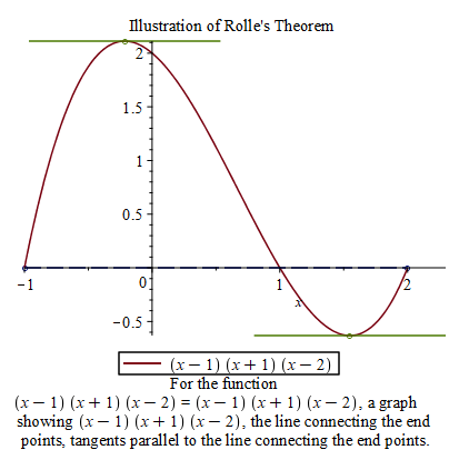

A demonstration of Rolle’s theorem

To find the values $x=c$. We solve the equation $f^{\prime }\left(x\right)=0$.

solve({D(f)(x)=0, x>-1, x<2}, x)

A generalization of Rolle’s theorem is the Mean Value Theorem.

If a function $f$ is continuous on the closed interval $[a,b]$ and differentiable on the open interval $(a,b)$, then there exists a point $c$ in $(a,b)$ such that $$f^{\prime }\left(c\right)=\frac{f\left(b\right)-f\left(a\right)}{b-a}$$ or equivalently, $$f\left(b\right)=f\left(a\right)+f^{\prime }\left(c\right)(b-a).$$

The subpackage Student[Calculus1] also provides a command MeanValueTheorem(f(x), x = a..b) to illustrate the Mean Value Theorem.

Example 4.3 Let $f\left(x\right)=(x-1)(x+1)(x-2)$. Graph the function $f\left(x\right)$ from $-2$ to $3$ indicate the points between $-2$ and $3$ where tangent line is parallel to the secant line passing through $(-2,f(-2\left)\right)$ and $(3,f(3\left)\right)$. Find the values $x=c$ where the tangent line is parallel to the secant line.

Solution. Define the function.

restart:
f:=x->(x-1)*(x+1)*(x-2)

Now let’s create the graph of the function and the horizontal tangent line.

with(Student[Calculus1]):
MeanValueTheorem(f(x), x = -2..3);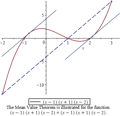

A demonstration of Mean Value Theorem

Find the slope msec of the secan line.

a:= -2;
b:= 3;
msec:=(f(a)-f(b))/(a-b);

Solve the equation $f^{\prime }\left(x\right)=$msec for $c$.

solve({D(f)(x)=msec, x>-2, x<3}, x)

Note that in Rolle’s theorem and Mean Value Theorem, the continuity and differentiability conditions are crucial.

Example 4.4 Consider the floor function $f\left(x\right)=\{\begin{array}{cc}1& x<0\\ 2& x\ge 0\end{array}$. Use a graph to show that there is no tangent line that is parallel to the secant line through $(-1,1)$ and $(1,2)$.

Solution. First define the function.

restart:
f := x->piecewise(x<0, 1, 2);

Now let’s find the second line.

a := -1; # left endpoint
b := 1; # right endpoint
msec:=(f(b)-f(a))/( b-a ); # slope of secant line
secline:=f(a) + msec*(x-a); # secant line

Plot the function and the secant line together.

plot([f(x), secline], x=a..b, discont=true);

Now try the MeanValueTheorem command.

with( Student[Calculus1] ):
MeanValueTheorem( f(x), a..b );

Exercise 4.3 Let $f\left(x\right)=\cos x$. Graph the function from $-\frac{2\pi }{3}$ to $\frac{4\pi }{3}$ and indicate the points in $[-\frac{2\pi }{3},\frac{4\pi }{3}]$ where the derivative $f^{\prime }\left(x\right)$ is $0$. Find the tangent points where the slope of the tangent line is $0$.

Exercise 4.4 Let $f\left(x\right)=x^4-3x^2+1$. Graph the function $f\left(x\right)$ from $-1$ to $2$ indicate the points between $-1$ and $2$ where tangent line is parallel to the secant line passing through $(-1,f(-1\left)\right)$ and $(2,f(2\left)\right)$. Find the tangent points where the tangent line is parallel to the secant line.

Exercise 4.5 Consider the floor function $f\left(x\right)=|x|$. Use a graph to show that there is no tangent line that is parallel to the secant line through $(-1,1)$ and $(2,2)$.

4.3 Derivatives and the Shape of a Graph

Given a function $f\left(x\right)$, we know that $f\left(x\right)$ is increasing on an interval if $f^{\prime }\left(x\right)>0$ on that interval and $f\left(x\right)$ is decreasing on an interval if $f^{\prime }\left(x\right)<0$ on that interval. By Mean Value theorem, $f\left(x\right)$ is a constant on an interval if $f^{\prime }\left(x\right)=0$ on that interval.

To determine over which interval a function $f\left(x\right)$ is increasing/decreasing, we need to find out the domain of $f^{\prime }\left(x\right)$ and the critical points and then use test points to determine the sign of $f^{\prime }\left(x\right)$.

Using first derivative, we can test local extrema at critical points.

Theorem 4.1 Suppose that $c$ is a critical point of a continuous function $f$.

1. If $f^{\prime }$ changes from positive to negative at $c$, then $f$ has a local maximum at $c$.
2. If $f^{\prime }$ changes from negative to positive at $c$, then $f$ has a local minimum at $c$.
3. If $f^{\prime }$ does not change signs at $c$, then $f$ has no local extremum at $c$.

Another method to determine local extremum is to use second derivative.

Theorem 4.2 Suppose $f$ is a twice differentiable function on an interval $I$.

1. If $f^{\prime \prime }>0$ over $I$, then $f$ is concave upward on $I$.
2. If $f^{\prime \prime }<0$ over $I$, then $f$ is concave downward on $I$.

Base on the observation on concavity, we have the following second derivative test.

Theorem 4.3 Suppose that $f^{\prime \prime }$ is continuous near $c$.

1. If $f^{\prime }\left(c\right)=0$ and $f^{\prime \prime }\left(c\right)>0$, then $f$ has a local minimum at $c$.
2. If $f^{\prime }\left(c\right)=0$ and $f^{\prime \prime }\left(c\right)<0$, then $f$ has a local maximum at $c$.

Example 4.5 Find local extrema, the intervals on which $f\left(x\right)=\frac{x}{x^2+1}$ is increasing or decreasing and the intervals on which $f\left(x\right)$ is concave up or concave down.

Solution. First we define the function and find the derivatives. f:=x->x/(x^2+1); df:=D(f); ddf:=D(D(f));

Now let’s find critical points using Student[Calculus1] subpackage. with(Student[Calculus1]): CriticalPoints(f(x),x)

Find the intervals of monotonicity (using test points).

df(t) # where t is a test point in an interval, you replace it by a number.

Determine local extrema and find values.

g(c) # suppose c is a critical point.

Find critical points of the derivative function $g^{\prime }\left(x\right)$ and determine intervals of concavity.

CriticalPoints(df(x),x);
ddf(t);     # evaluate the second derivative at a test point $t$.

From the outputs, we know that $f$ is decreasing on $(-\infty ,-1)\cup (1,\infty )$ and increasing on $(-1,1)$. It has a local minimum $f(-1)=-\frac{1}{2}$ and a local maximum $f\left(1\right)=\frac{1}{2}$.

The function is concave cup on $(-\sqrt{3},0)\cup (\sqrt{3},\infty )$ and concave down on $(-\infty ,-\sqrt{3})\cup (0,\sqrt{3})$.

Exercise 4.6 Let $f\left(x\right)=\sin x+\cos x$ be a function defined over the interval $[0,2\pi ]$. Find local extrema, the intervals on which $f$ is increasing or decreasing and the intervals on which $f\left(x\right)$ is concave up or concave down.

4.4 Limits at Infinity and Asymptotes

Limits at infinity can provide information on the end behaviors of a curve such as horizontal and vertical asymptotes.

When the limit of a function is an infinite limits, we will get a vertical asymptotes.

The function $f$ has a horizontal asymptote $y=b$ if $\underset{x\to \infty }{lim}f\left(x\right)=b$ or $\underset{x\to -\infty }{lim}f\left(x\right)=b$.

The function $f$ has a horizontal asymptote $x=a$ if $\underset{x\to a^{+}}{lim}f\left(x\right)=\infty$, $\underset{x\to a^{-}}{lim}f\left(x\right)=\infty$, $\underset{x\to a^{+}}{lim}f\left(x\right)=-\infty$ or $\underset{x\to a^{-}}{lim}f\left(x\right)=-\infty$.

The function $f$ has a slant asymptote $y=mx+b$ if $\underset{x\to \infty }{lim}\left(f\right(x)-(mx+b\left)\right)=0$ or $\underset{x\to -\infty }{lim}\left(f\right(x)-(mx+b\left)\right)=0$.

For rational functions, we have the following results. Suppose $p\left(x\right)=a_n{x}^n+\cdots +a_{1}x+a_0$ and $q\left(x\right)=b_m{x}^m+\cdots +a_{1}x+a_0$ $$\underset{x\to \infty }{lim}\frac{p\left(x\right)}{q\left(x\right)}=\{\begin{array}{cc}0& \text{if}n<m\\ \frac{a_n}{b_m}& \text{if}n=m\\ \pm \infty & \text{if}n>m\end{array}$$ In the last case, the sign agrees with the sign of $\frac{a_n}{b_m}$.

The limit at the negative infinity of a rational function is similar.

In Maple, to find limits, we use the command limit(f(x), x=a) or LimitTutor(f(x), x=a) supported by Student[Calculus1]. To find asymptotes, you may use the command Asymptotes(f(x), x) which is again supported by Student[Calculus1].

Example 4.6 Evaluate the following limits.

1. $\underset{x\to \infty }{lim}\sqrt{x^2+1}$,
2. $\underset{x\to -\infty }{lim}\frac{x^3-1}{\sqrt{9x^6-x}}$
3. $\underset{x\to \infty }{lim}x\sin \left(\frac{1}{x}\right)$.

Solution. Use LimitTutor to find limits step-by-step

with(Student[Calculus1]);
LimitTutor(sqrt(x^2+1), x=infinity);
LimitTutor((x^3-1)/(9*x^6-x), x=-infinity);
LimitTutor(x*sin(1/x), x=infinity);

Example 4.7 Find asymptote of the function $f\left(x\right)=\frac{x^3+2x^2-3x-1}{x^2-1}$ and plot the graph of $f$ and its asymptotes together with $x$ in $[-5,5]$ and $y$ in $[-10,10]$.

Solution. Define the function first.

restart:
f:=x-> (x^3+2*x^3-3*x-1)/(x^2-1);

Find and plot asymptotes. Here, it’s better to use implicitplot because vertical asymptotes are not functions of $x$.

with(Student[Calculus1]):
asym := Asymptotes(f(x), x);
with(plots):
asymplots := implicitplot(asym, x = -5 .. 5, y = -10 .. 10):

Plot the function $f$ and use display to put the graph and asymptotes together.

Grphf:=plot(f(x), x=-5..5, y=-10..10, discont=true):
display(asymplots, Grphf); # display is supported by the plots package.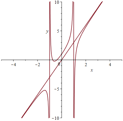

A graphs of rational functions with its asymptotes

Exercise 4.7 Evaluate the following limits.

1. $\underset{x\to \infty }{lim}\sqrt{x}\sin \left(\frac{1}{x}\right)$,
2. $\underset{x\to -\infty }{lim}\frac{\sqrt{9x^6+1}}{x^3+x}$.

Exercise 4.8 Find asymptote of the function $f\left(x\right)=\frac{2x^3-3x^2-5x+2}{x^2+1}$ and plot the graph of $f$ and its asymptotes together with $x$ in $[-5,5]$ and $y$ in $[-10,10]$.

Exercise 4.9 Find asymptote of the function $f\left(x\right)=\frac{8\sin x}{x^2+1}+\frac{x^2-x}{x^2-1}$ and plot the graph of $f$ and its asymptotes together with $x$ in $[-10,10]$ and $y$ in $[-20,20]$.

4.5 Curve Sketching

To plot the graph of a function in maple, we simply use the command plot(function, widows, options).

On the other hand, we can sketch the graph using calculus, more precisely, monotonicity, concavity, vertical asymptotes, horizontal asymptotes, periods, symmetries, local extrema, intercepts etc.

Example 4.8 Sketch and plot the graph of the function $g\left(x\right)=\frac{2x+1}{x-2}$.

Solution. First define the function

g:=x->(2*x+1)/(x-2)

Find the domain of the function.

solve((x-2)!=0, x)

Find the $x$-intercepts.

solve(g(x)=0, x)

Find the $y$-intercept

g(0)

Check whether $x=2$, where the function is undefined, is a vertical asymptote.

limit(g(x), x=2, left);
limit(g(x), x=2, right);

Find horizontal asymptotes

limit(g(x), x=infinity);
limit(g(x), x=-infinity);

Then we find derivative functions.

dg:=D(g);    # first derivative
ddg:=D(dg); # second derivative

Find all critical points. This can be done by finding using the Student[Calculus1] subpackage.

with(Student[Calculus1]):
CriticalPoints(g(x),x);

Find the intervals of monotonicity (using test points).

dg(t) # where t is a test point in an interval, you replace it by a number.

Determine local extrema and find values.

g(c) # suppose c is a critical point.

Find critical points of the derivative function $g^{\prime }\left(x\right)$ and determine intervals of concavity.

CriticalPoints(dg(x),x);
ddg(t);     # evaluate the second derivative at a test point $t$.

Sketch the graph using above obtained information and compare with Maple plot output.

plot(g(x), x=a..b) # Plot the function in the window [a, b].

Exercise 4.10 Sketch and plot the graph of the function $h\left(x\right)=\frac{x-1}{x+2}$.

Exercise 4.11 Sketch and plot the graph of the function $g\left(x\right)=x\sqrt{4-x}$.

4.6 Optimization Problems

To solve a optimization problem in Calculus, the key is to represent the quantity to be optimized by a function of other quantities and then find the extremum value using the extreme value theorem.

Example 4.9 Among rectangles with the same perimeter $16$ centimeters, there is one that has the largest area. Find the dimension of that rectangle.

Solution. Suppose the length is $x$ and the width is $y$. The area is a function of $x$ and $y$.

A:=(x, y)->x*y;

We know that the perimeter is $16$ which provides a relation between $x$ and $y$.

prm:=2x+2y=16;

Solve for $y$ and plug it in to the area function.

wd:=solve(prm, y);
y:=unapply(wd, x); # define y as a function of x
Ar:=unapply(A(x,y(x)),x); # Translate the area function into a function of x.

To find the maximum area, you may use maximize or using the following commands. Note that $x>0$.

Amx := max(Ar~(solve(D(Ar)(x) = 0, x))); # Find critical points, evaluate, and find the maximum.
xvalue := solve(Ar(x) = Amx, x); # Find the length x such that the area is the largest. 
yvalue := y(xvalue); # Find the width y such that the area is the largest.

Exercise 4.12 Find the rectangle with the minimal perimeter among rectangles with the area 36 square inches.

Exercise 4.13 Find the point on the parabola $y^2=2x$ that is closest to the point $(1,-4)$.

4.7 Antiderivatives

An antiderivative of a function $f$ over an interval $I$ is any function $F$ such that $F^{\prime }\left(x\right)=f\left(x\right)$ for all $x$ in $I$.

Antiderivatives are closely related to integration. In Maple, you may use int(f(x), x) or IntTutor(f(x), x) supported by Student[Calculus1] to find an antiderivative of $f\left(x\right)$.

Example 4.10 Find an antiderivative of the function $f\left(x\right)=x^3-\frac{1}{\sqrt{x}}$ by hand and by Maple respectively. Use diff to check your answer.

Solution. To find an antiderivative by hand, rewrite the function using negative rational exponent and apply the formula $$\frac{d}{dx}\left(\frac{1}{r+1}{x}^{r+1}\right)=x^r.$$

In this question, an antiderivative is $F\left(x\right)=\frac{1}{4}{x}^4-2\sqrt{x}$.

Define the function first.

restart:
f:=x->x^3-1/sqrt(x);

Find an antiderivative using int and using IntTutor for a step-by-step solution.

F:=int(f(x), x); # may define a function using unapply(int(f(x), x), x).

with(Student[Calculus1]):
TutorF:=IntTutor(f(x), x);

Verify using diff.

diff(F, x);
diff(TutorF, x);

Exercise 4.14 Find an antiderivative of the function $f\left(x\right)=x^2-3+8\sin \left(x\right)$ by hand and by Maple respectively. Use diff to check your answer.

Exercise 4.15 Find an antiderivative of the function $f\left(x\right)=\frac{x^3-2x+1}{\sqrt{x}}$ by hand and by Maple respectively. Use diff to check your answer.

Exercise 4.16 Find the most general antiderivative of the function $f\left(x\right)=\tan x\sec x+1$ by hand and by Maple respectively. Use diff to check your answer.