Topic 8 Calculus of Inverse Functions

8.1 Inverse Functions

Maple package Student[Calculus1] provides the following command

InversePlot(f(x), x = a..b);

which graphs the original function f(x)$f\left(x\right)$ and the inverse function f−1(x)$f^{-1}\left(x\right)$ together over the interval [a,b]$[a,b]$.

You will see clearly that the graphs of a function and its inverse are symmetric with respect to the line y=x$y=x$.

Example 8.1
1. Graph the function f(x)=x3−2$f\left(x\right)=x^3-2$, its inverse function, and the line y=x$y=x$ over the interval [−2,2]$[-2,2]$.

2. Find the inverse function.

Solution. One way to plot the function and its inverse together is to use the following command which is supported by the package Student[Calculus1].

  InversePlot(x^3-3, x = -2..2)

Here is the output in Maple

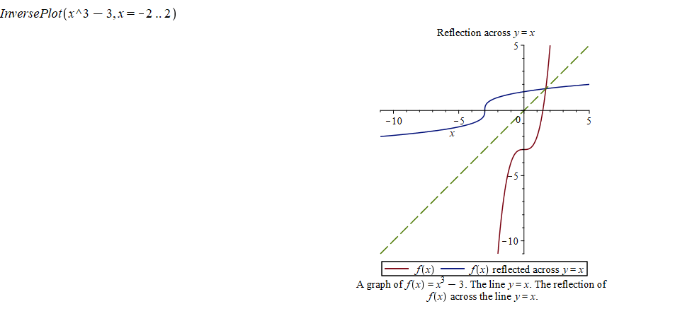
Graph of a pair of functions inverse to each other

Another way to plot the function f$f$ and its inverse g$g$ together uses the plot function.

  plot([f(x), g(x), x], x = -2 .. 4, y = -5 .. 5, color = [red, black, blue])

To find the inverse function, we replace f(x)$f\left(x\right)$ by y$y$, then switch x$x$ and y$y$, and solve for y$y$. In Maple, you may use the command solve(equation/inequality, variable) to solve an equation or an inequality (even system of equations/inequalities).

In this example, we may find the inverse function by type in the following command. Note I have switch x$x$ and y$y$.

solve(x=y^3, y)

To find the derivative of the inverse function of a function f$f$ at a given point x=a$x=a$, we may apply the formula (f−1)′(a)=1f′(f−1(a)). In Maple, we may use the following commands to calculate the value of the derivative function.

• Calculate the derivative of the function f.

diff(f(x), x)

• Find f−1(a) which is the solution of the equaiton f(x)=a.

solve(f(x)=a, x)

• Plug in the formula to evaluate.

eval(subs(x=f^{-1}(a), 1/f'(x)))

Example 8.2 Find (f−1)′(0), where f(x)=cos(x) and 0≤x≤π.

Solution. Find the derivative of f

diff(cos(x), x)

Find the value of f−1(0)

solve(cos(x)=0, x)

Apply the formula

eval(subs(x=Pi/2, -1/sin(x)))

Using Maple, we find (f−1)′(0)=−1.

Exercise 8.1 1. Graph the function f(x)=3+2sinx, its inverse function, and the line y=x over the interval [−2,2].

2. Find the value (f−1)′(5).

8.2 Logarithmic and Exponential Functions

8.2.1 Basic properties and graphs

The natural logarithmic function y=ln(x) is defined by ln(x)=∫x11tdt.

The natural exponential function y=ex is defined as the inverse function of y=ln(x).

From the definition, we have very important identities ln(ex)=xandelnx=x.

Using those two identities, we may define general exponential functions and general logarithmic function, and deduce the Law of Logarithms and Law of Exponents.

• For any positive number b≠1, we have bx=(elnb)x=exlnb.

• For any positive number b≠1, we define y=logbx to be the inverse function of y=bx

• By solving x=by for y, we find that logbx=lnxlnb. This identity is called the change of base property.

How do graphs of logarithmic functions and exponential functions look like?

Example 8.3 Graph the following functions together. y=lnx,y=ex,y=2x,y=log2x,y=x.

Solution. In Maple, the logarithm logbx is given by log[b](x). When b=e, you simply use ln(x) for lnx. When b=10, you may also use log(x) or log10(x) for log10x.

The exponent bx is given by b^x in Maple. When b=e, you may also use exp(x) to represent ex.

To graph the functions together with different colors, we use the following command

plot([ln(x), exp(x), 2^x, log[2](x), x], x=-5..5, color=[blue, green, purple, yellow, red])

Here is the output

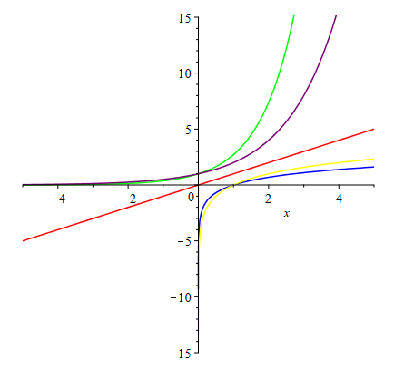
Logarithmic and exponential functions

Exercise 8.2 Graph the following functions together. y=log3x,y=3x,y=(1/3)x,y=log1/3x.

Find the pairs that are symmetric to each other with respect to a certain line.

Exercise 8.3 Graph the following functions together. y=0.5x,y=2x,y=5x.

Describe the monotonicity (increasing/decreasing) of the functions?

Fix an input x. Describe how y-values change when bases changes from small number to bigger number?

Exercise 8.4 Graph the following functions together. y=log0.5x,y=log2x,y=log5x.

Describe the monotonicity (increasing/decreasing) of the functions?

Fix an input x. Describe how y-values change when bases changes from small number to bigger number?

8.2.2 Differentiation and integration of logarithmic and exponential functions

In Maple, one way to do differentiation and integration is to use the Calculus Palette on the left side.

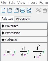
Calculus Palette in Maple

The other way is to use the commands diff(f(x), x) , int(f(x), x), and int(f(x), x=a..b).

Supported by the Student[Calculus1] package, Maple also provides the tutor commands DiffTutor() and IntTutor() which can show step-by-step solution of differentiation and integration.

Note you may also access tutor commands from the Start page (click the home button in the toolbar and look for Calculus).

Example 8.4 Find y′, where y=ln(x3+5x+1).

Solution. Using diff:

diff(ln(x^3+5*x+1), x)

We get y′=3x2+5x3+5x+1.

Type in (assume that with(Student[Calculus1]) was run)

DiffTutor(ln(x^3+5*x+1), x)

and hit enter you will see

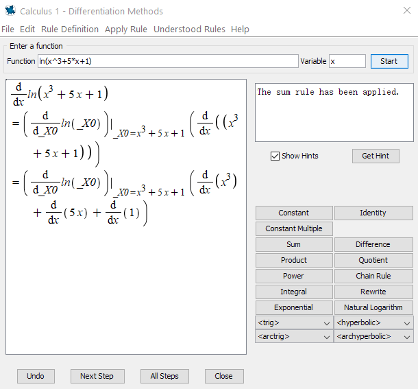
DiffTutor Example

By click Next Step or All Steps you will see detailed solution with rules used.

Example 8.5 Evaluate the integral ∫ex−1ex+1dx.

Solution. Using int:

int((exp(x)-1)/(exp(x)+1), x)

We get ∫ex−1ex+1dx=2ln(ex+1)−x+C.

Type in (assume that with(Student[Calculus1]) was run)

IntTutor((exp(x)-1)/(exp(x)+1), x)

and hit enter you will see

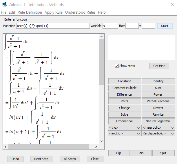
IntTutor Example

By click Next Step or All Steps you will see detailed solution with rules used.

Exercise 8.5 Find the derivative dydx, where y=ln|cosx|

Exercise 8.6 Find the derivative dydx, where y=xcosx

Exercise 8.7 Evaluate the integral ∫(e4x+e2x)e3xdx

Exercise 8.8 Evaluate the integral ∫23xdx

8.3 Solve differential equations

In Maple, you may solve the equation y′(x)=ky(x)+c (which is called an ODE) using the command dsolve({ics, eq}), where ics stands for initial condition y(0)=c and eq stands for the differential equation. Without the ics, dsolve will provide a general solution.

Example 8.6 Find the function f(x) which satisfies the differential equation f′(x)=kf(x) with f(0)=5 and f(2)=3.

Solution. Use the following command

dsolve({f(0)=5, f'(x)=k f(x)})

we get f(x)=5ekx.

To find k, we solve the equation 3=5e2k by

solve(3=5*e^(2*k), k)

which shows that k=ln3−ln52≈−0.255. Here we use evalf(%) (% represents the previous result) to get the approximation.

So the function f is given by f(x)=5ex(ln3−ln5)2≈5e−0.255x.

Exercise 8.9 Find the function y which satisfies the differential equation y′(x)=ky(x) with y(0)=2 and y(5)=11.

8.4 Inverse Trigonometric Functions

8.4.1 Domains and Ranges

To define the inverse function, the original function must be a one-to-one function. For a trigonometric function, we have to restrict the function over a specific domain to ensure that the function is one-to-one. For simplicity, we pick domains near the origin for trigonometric functions. To be more precise, we consider the following trigonometric functions: y=sinx,−π/2≤x≤π/2  and −1≤y≤1;

y=cosx,0≤x≤π  and −1≤y≤1;

y=tanx,−π/2<x<π/2  and −∞<y<∞.

Their inverse functions are

y=arcsinx,−π/2≤y≤π/2  and −1≤x≤1;

y=arccosx,0≤y≤π  and −1≤x≤1;

y=arctanx,−π/2<y<π/2  and −∞<x<∞.

To see the graphs of the functions, we may use the plot(f(x), x = a..b, opts) command. Or, to graph f, f−1 and y=x together, we may also use the command InversePlot(f(x), x = a..b, opts) supported by the package Student[Calculus1].

Example 8.7 Graph the following functions together. y=tanx,y=arctanx,y=x.

Solution. #load the package Student[Calculus1]". with(Student[Calculus1]) #plot the functions InversePlot(tan(x),x=-Pi/2..Pi/2)

Here is the output

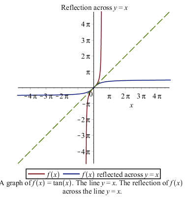
Tangent and arctangent functions

Exercise 8.10 Graph the following functions together over an appropriate domain. y=cotx,y=arccotx,y=x.

What’s the domain and range of y=arccotx?

8.4.2 Differentiation and integration of inverse trigonometric functions

In the section {#Differentiation and integration of logarithmic and exponential functions}, we learned to how use Maple to learn differentiation and integration.

Now let find derivatives and integrals of some inverse trigonometric functions.

Example 8.8 Find y′, where y=arccotx.

Solution. Surely, we may use diff or DiffTutor to find the derivative.

Here let’s me introduce to you another command implicitdiff.

We’ve learned that (see {#Inverse Functions}) to find the inverse function, we switch x and y and then solve for y. When finding the derivative, we don’t have to solve for y instead, we want y′ which is implicitly defined by an equation. In this case, we have x=arccoty.

Enter the following commands in Maple, you will find y′=−1x2+1.

implicitdiff(x=cot(y), y, x)
subs(cot(y) = x, %)

where % is a ditto operator that allows you to refer to a previously computed result in Maple.

Exercise 8.11 Find the derivative of y=arcsecx

Exercise 8.12 Find the derivative of y=arccscx

For integrals of inverse trigonometric function, you may need the method of integration by parts.

Use DiffTutor to find antiderivatives of inverse trigonometric functions.

Exercise 8.13 Evaluate the integral ∫arcsinxdx

Exercise 8.14 Evaluate the integral ∫arctanxdx

Exercise 8.15 Evaluate the integral ∫secxdx

8.5 L’Hospital’s Rule

In Maple, supported by the package, Student[Calculus1], the command LimitTutor can show step-by-step solutions of evaluating limits.

Example 8.9 Evaluate the limit limx→∞(1+x)1/ln(x)

Solution. # load the package Student[Calculus1]. with(Student[Calculus1]) #Find the limit step-by-step using LimitTutor LimitTutor((1+x)^(1/ln(x)), x = infinity)

Exercise 8.16 Estimate the limit limx→1x2−2x+1x2−x by graphing and verify your estimation.

Exercise 8.17 Evaluate the limit limx→∞x−ln(x).

Exercise 8.18 Evaluate the limit limx→∞xtan(1x).