Topic 2 Limits
2.1 Understand limits using tangent lines
Intuitively, the limit of a function \(f\) at \(x=a\) is a fixed value \(L\) that values of the function \(f(x)\) approach as the values of \(x\) \((\ne a)\) approach \(a\).
The slope of a tangent line to the graph of a functions is a limit of slopes of secant lines. This can be visualized easily using Maple with the support of the package Student[Calculus1].
Like predefined functions in Maple, package consists of predefine commands for Maple. The package Student serves for studying Calculus and other subject interactively. The subpackage Student[Calculus1] focus mainly on Calculus as the name indicated.
As different package has different focus and serves for different purpose, Maple won’t load a specific package until you run the command with(package_name). For example, the command
with(Student[Calculus1]) will load the subpackage Calculus1.
Example 2.1 Observe how do secant lines of the function \(f(x)=x^3-2\) approach to the tangent line at \(x=1\).
Solution. Load the Student[Calculus1] package using with().
with(Student[Calculus1])Use TangentSecantTutor from the loaded package to observe changes of secant lines.
TangentSecantTutor(x^3-1, x=1)Exercise 2.1 Explore the package Student, in particular the subpackage Student[Calculus1].
You can use the command ?Student to get help.
TangentSecantTutor command.
2.2 Estimate limits numerically or graphically
To estimate a limit \(\lim\limits_{x\to a}f(x)\) numerically, one may pick some values close to \(a\) and evaluate the function. In Maple, the calculation can be done by using the repetition statement for counter in array do statement end to;.
Solution. First, we pick some values close to 0, for example -0.01, -0.001, -0.0001, 0.01, 0.001, 0.0001 and assign them to an expression.
sq:=[-0.01, -0.001, -0.0001, 0.0001, 0.001, 0.01]Now we find the function values using two new commands instead of defining the function a priori.
for t in sq do evalf(subs(x=t, sin(x)/x)) end do;Graphs provide visual intuition which helps understand and solve problems. Recall, the command plot(expression, domain, option) produces a graph of the function defined by the expression over your choice of domain.
Example 2.3 Determine whether the limit \(\lim\limits_{x\to 0}\frac{1}{1- \cos x}\) exists.
Solution.
Apply the plot function to the expression over the domain \((-0.5, 0.5)\).
plot(1/(1-cos(x)), x=-0.5..0.5)The graph shows that the function \(y=\frac{1}{1- \cos x}\) goes to \(\infty\) when \(x\) approaches \(0\). So the limit is an infinite limit.
Exercise 2.2 Estimate the limit \(\lim\limits_{t \to 0}\frac{1-\cos x}{x}\) numerically.
Exercise 2.3 Determine whether the limit \(\lim\limits_{x \to 1}\frac{\sin x}{|x-1|}\) exists using the graph.
2.3 Evaluate limits
Maple provides the following command to evaluate a limit
limit(function, position, direction)
The direction may be omitted when evaluating a two-side limit.
Example 2.4 Determine whether the limit \(\lim\limits_{x\to 0}\frac{|x|}{x}\) exists.
Solution. You may find the left and right limits using the following commands.
limit(abs(x)/x, x=0, left);
limit(abs(x)/x, x=0, right);
It turns out that \(\lim\limits_{x\to 0}\frac{|x|}{x}\) does not exist because the left limit and the right limit are different.
Example 2.5 Evaluate the limit \(\lim\limits_{h\to 0}\dfrac{f(x+h)-f(x)}{h}\), where \(f(x)=\dfrac{1}{x}\).
Solution. The limit can be obtained using the following command.
limit((1/(x+h)-1/x)/h, h=0)Exercise 2.4 Determine whether the limit \(\lim\limits_{x\to 1/2}\dfrac{2x-1}{|2x^3-x^2|}\) exists.
Exercise 2.5 Evaluate the limit \(\lim\limits_{t\to 0}\dfrac{\sqrt{x+t}-\sqrt{x}}{t}\).
2.4 Learn limit laws using LimitTutor
Suppose the limits of two functions \(f\) and \(g\) at the same point \(x=a\) exist (equal finite numbers). Then the limit operation commutes with addition/subtraction, multiplication/division and power.
In Maple, you may use the command LimitTutor(function, position, direction), which is again supported by the subpackage Student[Calculus1], to learn how to evaluate a limit using limit laws and theorems.
Note that LimitTutor employs all limits laws available in Calculus including the L’Hopital rule which will be taught in Calculus 2.
To avoid L’Hopital’s Rule when using LimitTutor, it’s better to rationalize the expression first. For radicals, you may use the command rationalize(). When rationalization involves trigonometric functions, we will have to do it “manually” using the command simplify(expr, trig). For example, the following command will output \(sin^x(x)\).
simplify((1 - cos(x))*(1 + cos(x)), trig)Example 2.6 Evaluate \(\lim\limits_{x\to 0}\dfrac{1-\cos x}{x}\).
Solution. We will do the calculations in two ways.
Load the subpackage Student[Calculus1] if it was not loaded.
with(Student[Calculus1])Method 1: Use the following command to evaluate the limit.
LimitTutor((1-cos(x))/x, x=0)You will see an interactive windows pop out. You can choose the see the procedure step-by-step.
Method 2: Rationalize the numerator first and then evaluate the limit using LimitTutor f:=simplify((1 - cos(x))(1 + cos(x)), trig)/(x(1 + cos(x))); LimitTutor(f, x = 0);
Can you tell the difference?
Exercise 2.6
Evaluate \(\lim\limits_{x\to 0}\dfrac{(x+2)(\cos x-1)}{x^2-x}\) using LimitTutor.
2.5 Squeeze Theorem
Comparison is a very useful tool in problem solving. Squeeze theorem is such an example
Theorem 2.1 (Squeeze Theorem) Suppose that \[ f(x)\leq g(x)\leq h(x) \] and \[ \lim\limits_{x\to c}f(x)=L=\lim\limits_{x\to c}h(x). \] Then \[ \lim\limits_{x\to c}g(x)=L. \]
Let’s use Maple to understand the statement.
Example 2.7 Graph the functions \(f(x)=-x\), \(g(x)=x\cos\frac1x\) and \(h(x)=x\) in the same coordinate system. What’s the limit of \(g(x)\) as \(x\) approaches \(0\).
Solution.
We use the plot() command to graph the functions together.
plot([-x, x*cos(1/x), x], x=-1..1, discont, color=[red, blue, red])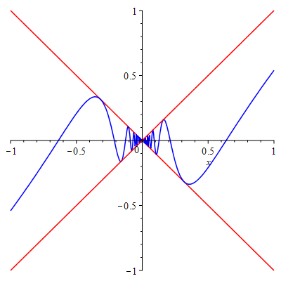
Squeeze Theorem demonstration
From the graph, we see that the \(\lim\limits_{x\to c}f(x)=0\) as it is squeezed by two limits which are both \(0\).
Exercise 2.7 Graph the functions \(f(x)=-x\), \(g(x)=x\sin\frac1x\) and \(h(x)=x\) in the same coordinate system. What’s the limit of \(g(x)\) as \(x\) approaches \(0\).
2.6 Continuity
A function \(f\) is continuous at \(x=a\) if \(f(a)\) is defined and \(\lim\limits_{x\to a}f(x)=f(a)\). Intuitively, a function is continuous if the graph has no hole or jump.
Example 2.8 Use graph to determine if the function \[ f(x)= \begin{cases} x & x\le -1 \\ 1/(x-1) & -1<x<1\\ 3-x & 1\le x\le 2\\ \sin(x - 2) + 1 & x>2\\ -2 & x=2 \end{cases} \] is continuous over \((-\infty, \infty)\). Find the discontinuities and verify them using the definition and properties of continuity.
Solution. First we define the function.
f := x -> piecewise(x <= -1, x, -1 < x and x < 1, 1/(x - 1),
1 <= x and x < 2, 3 - x, 2 < x, sin(x - 2) + 1, -2)
We first check visually whether the graph has holes or jumps.
plot(f(x), discont=[showremovable], x=-5..5, smartview=true)In the above command, the option discont = [showremovable] is used to show removable discontinuities.
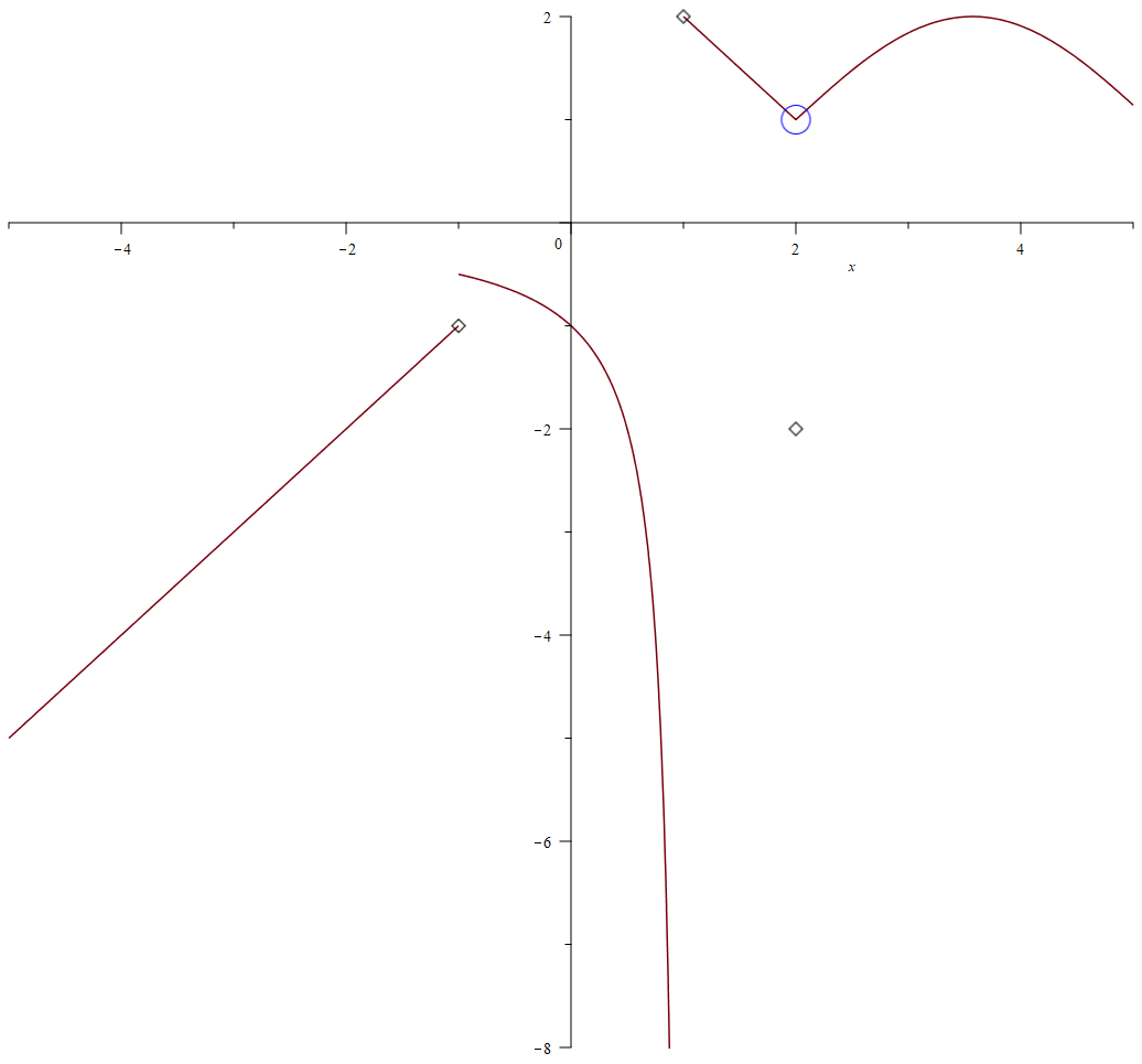
An example shows three types of discontinuities
From the graph, we can tell that the function has discontinuities which can also be found using Maple.
discont(f(x), x)Maple gives three discontinuities \(\{-1, 1, 2\}\).
Let’s first find limits at all three values.
discontset:=[-1, 1, 2];
for a in discontset do limit(f(x), x=a) end do;
You will find that limits do not exist at \(-1\) and \(1\). The limit at \(2\) is \(1\). However, \(g(2)=-2\). So \(f\) has three discontinuities at \(x=-1\), \(x=1\) and \(x=2\).
2.7 Continuity and Limit of a Composite Function
Continuous functions behave under composition. The composition of continuous functions is still continuous over its domain. More generally,
In general, the limit does not commute with composition.
Example 2.9 Let \[ f(x)=x^3\quad \text{and}\quad g(x)= \begin{cases} 1 & x=0\\ 2x-1 & \text{otherwise} \end{cases} \]
Verify that \[ \lim_{x\to 0}f(g(x))=f(\lim_{x\to 0}g(x)). \]
Is is true that \[ \lim_{x\to 0}g(f(x))=g(\lim_{x\to 0}f(x))? \]Solution. We first define \(f\) and \(g\) in Maple
f:=x->x^2;
g:=x->piecewise(x=0, 1, 2x-1);
Evaluate limits for \(f\circ g\).
limit(f(g(x)), x=0);
f(limit(g(x), x=0));
The results verify that the limit commutes with composition if the outside function is continuous.
Evaluate limits for \(g\circ f\)
limit(f(g(x)), x=0);
f(limit(g(x), x=0));
The results show that the limit may not commute with composition if the outside function is not continuous.
Exercise 2.9 Find three functions \(f\), \(g\), \(h\) and a value \(c\) such that \(f(g(x))\) is continuous, \[ \lim\limits_{x\to c}f(h(x))=f(\lim\limits_{x\to c}h(x)) \] and \[ \lim\limits_{x\to c}h(g(x))\neq h(\lim\limits_{x\to c}g(x)). \]
2.8 Intermediate Value Theorem
A very important result about continuity is the intermediate value theorem (IVT for short).
Theorem 2.3 (Intermediate Value Theorem) Let \(f\) be a function continuous over the interval \([a, b]\). Suppose that \(f(a)\neq f(b)\) and \(N\) is a number between \(f(a)\) and \(f(b)\). Then there exists a number \(c\in (a, b)\) such that \(f(c)=N\).
In particular, if \(f(a)f(b)<0\) then there exists a number \(c\) such that \(f(c)=0\).
Example 2.10 Determine whether the equation \[ \sin^2x+2x-1=0 \] has the solution in \((-1, 1)\). Estimate the solution if it exists.
Solution. We first use the left hand side of the equation to define a function \(eql\).
eql:=x->sin(x)^2 + 2*x - 1
Now lets verify that \(eql\) is continuous over \([-1,1]\) using the command iscont().
iscont(eql(x), x=-1..1)The result is True. We may apply the IVT. Let’s check if the value \(eql(-1)\cdot eql(1)<0\).
evalf(eql(-1)*eql(1))Here evalf() convert the symbolic answer to the (approximate) numerical value.
Since the product is negative, applying the IVT, we know there exists a solution between \((-1, 1)\).
This can also be seen from the graph using the command.
plot(eql(x), x=-1..1)To estimate the solution, you may use the Maple command
evalf(solve(eql(x) = 0, x))or you may repeatedly apply IVT to find an approximate solution.
m:=10;
a:=-1;
b:=1;
for n from 1 to m do
    c[n] := (a + b)/2;
    if evalf(eql(c[n])*eql(a)) < 0 then
        b := c[n];
    else
        a := c[n];
    end if;
    evalf(eql(c[n]));
end do;
Exercise 2.10 Find an integer \(k\) such that the equation \[ \cos^2x + 3x - 2=0 \] has a solution in \((k, k+1)\). Estimate the solution.